44 pivot table multiple row labels

How to Create Pivot Table in Excel: Beginners Tutorial Notice the drop down button next to Rows Labels. This button allows us to sort/filter our data. Let's assume we are only interested in Alfreds Futterkiste Click on the Row Labels drop down list as shown below Remove the tick from (Select All) Select Alfreds Futterkiste Click on OK button You will get the following data 2-Dimensional pivot tables One Weird Trick for Smarter Map Labels in Tableau - InterWorks Set the transparency to zero percent on the filled map layer to hide the circles. Turn off "Show Mark Labels" on the layer with "circle" as the mark type to avoid duplication. If you don't want labels to be centered on the mark, edit the label text to add a blank line above or below. Experiment with the text and mark sizes to find the ...

How To Create A Pivot Table In Excel - Naukri Learning The data should be organized in rows and columns where each column has a title. To create a pivot table, we follow these steps: Step 1 - Insert your data on the excel sheet Click any cell in the source data and go to the Insert tab. Click the PivotTable button inside the Tables group.

Pivot table multiple row labels

VBA Excel pivot table value "Count of Number" replaces row "Number" Follow-up: My actual pivot table contains four columns, with Number being 2 and "Count of Number" being 3. If I add the value (consolidation function) for a specific field before adding the field (row) itself, it works correctly. linkedin-skill-assessments-quizzes/microsoft-excel-quiz.md at ... - GitHub Q69. The PivotTable below has one row field and two column fields. How can you pivot this table to show the column fields as subtotals of each value in the row field? On the PivotTable itself, drag each Average field into the row fields area. Right-click a cell in the PivotTable and select PivotTable Options > Classic PivotTable layout. Pivot Chart in Vue Pivot Table component - Syncfusion In pivot table component, pivot chart would act as an additional visualization component with its basic and important characteristic like drill down and drill up, 15+ chart types, series customization, axis customization, legend customization, export, print and tooltip. Its main purpose is to show the pivot data in graphical format.

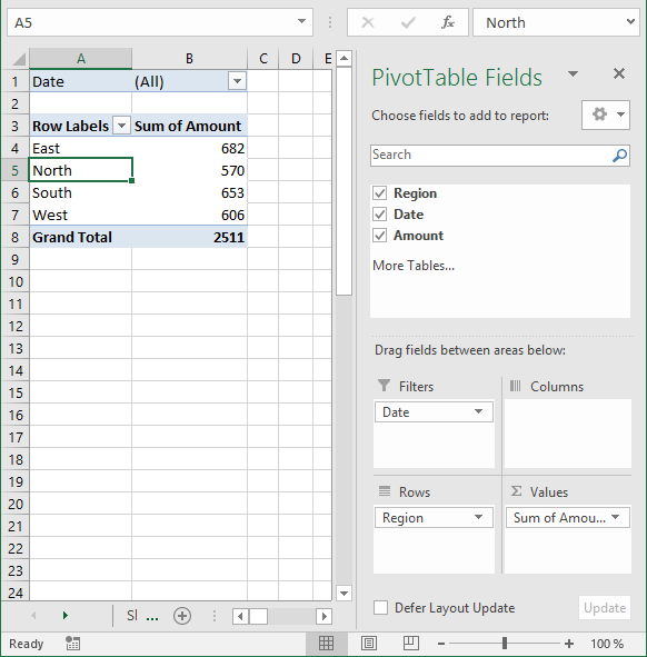
Pivot table multiple row labels. Excel Pivot Table tutorial - Ablebits To do this, in Excel 2013 and higher, go to the Insert tab > Charts group, click the arrow below the PivotChart button, and then click PivotChart & PivotTable. In Excel 2010 and 2007, click the arrow below PivotTable, and then click PivotChart. 3. Arranging the layout of your pivot table report PDF Pivot Data In A Pivottable Or Pivotchart Report Lmu Sorting Data in the Pivot Table with Pivot AutoSort. Another way to sort data in the Pivot table is to use the AutoSort option in the Pivot table. If we want to sort the table ascending by Row labels (Salesman), we need to click on the AutoSort icon next to the Row Labels, choose Sort A to Z and click OK: ... Turning Off Automatic Sorting in PivotTables (Microsoft Excel) Follow these steps: Create your PivotTable as you normally would. Click the down-arrow at the right of the Column Labels cell or the Row Labels cell, depending on whether you want to affect column or row sorting. Excel displays some options. Choose More Sort Options. Excel displays the Sort dialog box. What Is An Excel Pivot Table And How To Create One Creating A Pivot Table Follow these easy steps to create the table. #1) Click anywhere on the data table you just created. #2) Go to Insert -> PivotTable #3) Create PivotTable dialog will appear as shown below. The first section will give you the details about the table that you want to analyze.

Pivot Table Grouping, Ungrouping And Conditional Formatting #1) Select the entire column under the Sum of Total column in the pivot table. #2) Navigate to Home -> Conditional Formatting #3) Select Top/Bottom Rules -> Bottom 10 items. #4) In the dialog reduce the count to 3 (since we want just the bottom 3) and you can choose any highlighter from the drop-down. How to use Table Spreadsheet macro - StiltSoft Docs - Table Filter and ... Reusing of the Table Spreadsheet macro. Save data in the Table Spreadsheet macro via File->Save (to have a generated name) or via File->Save As (to name it yourself). Get to the page you wish for the spreadsheet's new location. Open the page in the edit mode and insert the Table Spreadsheet macro. How to: Filter Items in a Pivot Table - DevExpress To enable the capability to apply multiple filters to a single row or column field, set the PivotBehaviorOptions.AllowMultipleFieldFilters property to true. By default, this property is false and if you try to apply more than one filter to a PivotTable field, only the last specified filter will be applied. View Example PivotTableFilterActions.cs Working with "Check All That Apply" Survey Data (Multiple Response Sets ... From left to right, the columns of this table show: First column: The name or label of the multiple response set. Second column: The variable names or variable labels (if assigned) of the variables in the multiple response set. N: The number of cases who selected that response option. Notice that these values match the valid values in the ...

Pivot table enhancements - EPPlus Software EPPlus 5.4 adds support for pivot table filters, calculated columns and shared pivot table caches. The following filters are supported. Item filters - Filters on individual items in row/column or page fields. Caption filters (label filters) - Filters for text on row and column fields. Date, numeric and string filters - Filters using various ... r - Label or Highlight Specific Rows in ggplot2 - Stack Overflow Row axis titles are much too long and too many to look good There are only 53 bin_level rows with a 1 (of 1045 total), so why does it look like a LOT more red than there should be? I want the red labels (bin_level =1's) at the top of the plot, and the mix of black/red makes me think my arrange(bin_level) piece isn't working right. How to Set Up Excel Pivot Table for Beginners A pivot table is a quick way to show a summary for many rows of data. It is a flexible alternative to a structured worksheet report that has typed headings, and formulas to calculate the totals. There are a few things to do though, before you build a pivot table. Being prepared can save you lots of time and troubleshooting later! 1. Excel: Group rows automatically or manually, collapse and ... - Ablebits For this, we select rows 10 to 16, and click Data tab > Group button > Rows. That set of rows is now grouped too: Tip. To create a new group faster, press the Shift + Alt + Right Arrow shortcut instead of clicking the Group button on the ribbon. 2. Create nested groups (level 2)

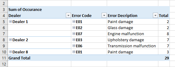
Pivot Table Multiple Row Labels Side By Side | Decorations I Can Make

Excel Pivot Table DrillDown Show Details Right-click the pivot table's worksheet tab, and then click View Code. That opens the Visual Basic Explorer (VBE). Paste the copied code onto the worksheet module, below the Option Explicit line (if there is one), at the top of the code module (optional) Paste the copied code onto the worksheet module for any other pivot tables in your workbook

How to Sort Pivot Table Row Labels, Column Field Labels and Data Values with Excel VBA Macro ...

Grouping or summarizing rows - Power Query | Microsoft Docs Enter the formula Table.Max([Products], "Units" ) under Custom column formula. The result of that formula creates a new column with [Record] values. These record values are essentially a table with just one row. These records contain the row with the maximum value for the Units column of each [Table] value in the Products column.

How To Make Awesome Ranking Charts With Excel Pivot Tables - Moz

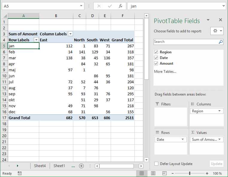
Work with PivotTables in Office Scripts - Office Scripts A PivotTable can have as many or as few of its fields assigned to these specific hierarchies. A PivotTable needs at least one data hierarchy to show summarized numerical data and at least one row or column to pivot that summary on. The following code snippet adds two row hierarchies and two data hierarchies. TypeScript

Insert Subtotals to a Pivot Table - Free Microsoft Excel Tutorials

What is pivot table | Easy World Change the style of your PivotTable Click anywhere in the PivotTable to show the PivotTable Tools on the ribbon. Click Design, and then click the More button in the PivotTable Styles gallery to see all available styles. Pick the style you want to use. If you don't see a style you like, you can create your own. Tags What is pivot table Older Post

Discover Pivot Tables – Excel’s most powerful feature and also least known

How to perform Pivot and Unpivot of DataFrame in Spark SQL Step 2: Pivot Spark DataFrame Spark SQL provides a pivot () function to rotate the data from one column into multiple columns (transpose row to column). It is an aggregation where one of the grouping columns values is transposed into individual columns with distinct data.

Pivot Table Row Labels In the Same Line - Beat Excel!

How to Sort Pivot Table Manually? - Excel Unlocked However, to manually sort the rows:- Click on the button next to Row Labels in cell B3. Click on More Sort Options from there and choose the Manual Sort option. This opens the Sort Dialog box for Pizza Sizes. Choose the first option for Manual Sort. This enables the Manual Sort and now we need to actually manually sort the pivot table rows.

Naming Columns | CLEARIFY

How to use Table Excerpt and Table Excerpt Include macros labels The macros improve the performance of pages storing large tables and let you use the original tables for any purpose, including filtering, building multiple charts and pivot tables. #14 - Building multiple pivot tables and charts from the single table Why should I use these macros? When you build multiple pivot tables and charts from table

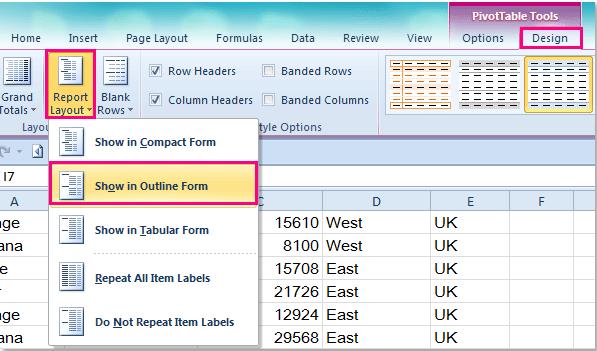
How to repeat row labels for group in pivot table?

Excel Articles - dummies Excel Excel 2010 All-in-One For Dummies Cheat Sheet. Cheat Sheet / Updated 04-20-2022. As an integral part of the Ribbon interface used by the major applications included in Microsoft Office 2010, Excel gives you access to hot keys that can help you select program commands more quickly. As soon as you press the Alt key, Excel displays the ...

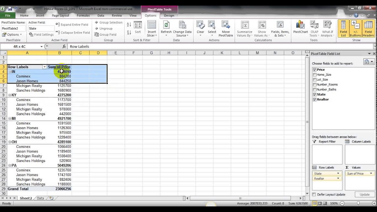
Pivot table row labels in separate columns • AuditExcel.co.za

3 Ways to Preserve 'Percent of Total' within Filtered Dimensions This will ensure that our data is filtered after the table calc occurs. Step 4: Move the index filter field onto the filters shelf with the value TRUE. Points to Ponder: Table calcs can break. Our filter is being applied after Tableau has already run the database query, so we're pulling everything into memory and doing less with the result.

Multiple Row Filters in Pivot Tables - YouTube

Solved: Pivot Table Row Headers - Qlik Community - 1918577 While creating a Pivot table and when we add the dimensions as rows in Pivot table all the dimension names were getting added next to each other in the Pivot table header (row header coming empty) insisted of each row header, because of this user feeling very difficult to read the table.

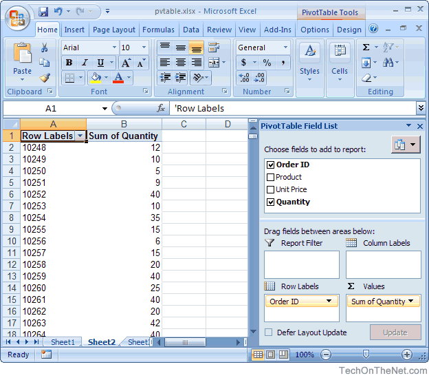
MS Excel 2007: How to Create a Pivot Table

excel transpose multiple rows in group to columns Step 1: Determine the rows and columns of data. 5. On your keyboard, press Alt + Q to return to the worksheet. Press with left mouse button on "Add Chart Element" button.

How to Show the Percentage of Row Total in the Pivot Table - MS Excel | Excel In Excel

Pivot Chart in Vue Pivot Table component - Syncfusion In pivot table component, pivot chart would act as an additional visualization component with its basic and important characteristic like drill down and drill up, 15+ chart types, series customization, axis customization, legend customization, export, print and tooltip. Its main purpose is to show the pivot data in graphical format.

Pivot Table Row Labels In the Same Line - Beat Excel!

linkedin-skill-assessments-quizzes/microsoft-excel-quiz.md at ... - GitHub Q69. The PivotTable below has one row field and two column fields. How can you pivot this table to show the column fields as subtotals of each value in the row field? On the PivotTable itself, drag each Average field into the row fields area. Right-click a cell in the PivotTable and select PivotTable Options > Classic PivotTable layout.